Tutorial 3: Spiking Networks

Up to this point we’ve created networks of neurons and synapses which only operate in the non-spiking regime. In this tutorial, we will create a network of spiking neurons and populations, and record activity with spike monitors.

Step 1: Imports

# Add the library to the path
# If jupyter cannot find SNS-Toolbox
import os
import sys
module_path = os.path.abspath(os.path.join('..'))
if module_path not in sys.path:
    sys.path.append(module_path)

# Import packages and modules for designing the network
from sns_toolbox.networks import Network
from sns_toolbox.connections import SpikingSynapse
from sns_toolbox.neurons import SpikingNeuron
from sns_toolbox.renderer import render

# Import packages and modules for simulating the network
import numpy as np
import matplotlib.pyplot as plt
from sns_toolbox.plot_utilities import spike_raster_plot # This module is necessary for plotting spike rasters

Step 2: Design the First Network

# Create spiking neurons with different values of 'm'
threshold_initial_value = 1.0
spike_m_equal_0 = SpikingNeuron(name='m = 0', color='aqua',
                                threshold_time_constant=5.0,  # Default value of tau_m (ms)
                                threshold_proportionality_constant=0.0,  # Default value of m
                                threshold_initial_value=threshold_initial_value)  # Default value of theta_0 (mV)
spike_m_less_0 = SpikingNeuron(name='m < 0', color='darkorange',
                               threshold_proportionality_constant=-1.0)
spike_m_greater_0 = SpikingNeuron(name='m > 0', color='forestgreen',
                                  threshold_proportionality_constant=1.0)

# Create a spiking synapse
synapse_spike = SpikingSynapse(time_constant=1.0)    # Default value (ms)

# Create a network with different m values
net = Network(name='Tutorial 3 Network Neurons')
net.add_neuron(spike_m_equal_0, name='m=0')
net.add_neuron(spike_m_less_0, name='m<0')
net.add_neuron(spike_m_greater_0, name='m>0')

# Add an input current source
net.add_input(dest='m=0', name='I0', color='black')
net.add_input(dest='m<0', name='I1', color='black')
net.add_input(dest='m>0', name='I2', color='black')

# Add output monitors (some for the voltage, some for the spikes)
net.add_output('m=0', name='O0V', color='grey')
net.add_output('m=0', name='O1S', color='grey', spiking=True)  # Records spikes instead of voltage
net.add_output('m<0', name='O2V', color='grey')
net.add_output('m<0', name='O3S', color='grey', spiking=True)  # Records spikes instead of voltage
net.add_output('m>0', name='O4V', color='grey')
net.add_output('m>0', name='O5S', color='grey', spiking=True)  # Records spikes instead of voltage

render(net)

Step 3: Design the Second Network

pop_size = 5
net_pop = Network(name='Tutorial 3 Network Populations')
initial_values = np.linspace(0.0,threshold_initial_value,num=pop_size)
net_pop.add_population(spike_m_equal_0, shape=[pop_size], color='red', name='Source',initial_value=initial_values)
net_pop.add_population(spike_m_equal_0, shape=[pop_size], color='purple', name='Destination',initial_value=initial_values)
net_pop.add_input(dest='Source', name='I3', color='black')
net_pop.add_connection(synapse_spike, 'Source', 'Destination')
net_pop.add_output('Source', name='O6S', color='grey', spiking=True)
net_pop.add_output('Source', name='O7V', color='grey', spiking=False)
net_pop.add_output('Destination', name='O8S', color='grey', spiking=True)
net_pop.add_output('Destination', name='O9V', color='grey', spiking=False)

render(net_pop)

Step 4: Combine the Networks

In order for easier simulation, we can combine these two networks into one larger network so that we only need one input and output vector.

net_comb = Network(name='Tutorial 3 Network Combined')
net_comb.add_network(net)
net_comb.add_network(net_pop)

render(net_comb)

Step 5: Simulate the Networks

dt = 0.01
t_max = 10

t = np.arange(0, t_max, dt)
inputs = np.zeros([len(t), net_comb.get_num_inputs()]) + 20      # getNumInputs() gets the number of input nodes in a network
data = np.zeros([len(t), net_comb.get_num_outputs_actual()])    # getNumOutputsActual gets the number of accessible output
                                                            # nodes in a network (since this net has populations, each
                                                            # population has n output nodes)
# Compile to numpy
model = net_comb.compile(backend='numpy', dt=dt, debug=False)

# Run for all steps
for i in range(len(t)):
    data[i,:] = model(inputs[i,:])
data = data.transpose()

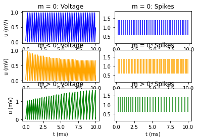
Results from First Network

plt.figure()
plt.subplot(3,2,1)
plt.title('m = 0: Voltage')
plt.plot(t,data[:][0],color='blue')
# plt.xlabel('t (ms)')
plt.ylabel('u (mV)')
plt.subplot(3,2,2)
plt.title('m = 0: Spikes')
spike_raster_plot(t, data[:][1],colors=['blue'])
# plt.xlabel('t (ms)')
plt.subplot(3,2,3)
plt.title('m < 0: Voltage')
plt.plot(t,data[:][2],color='orange')
# plt.xlabel('t (ms)')
plt.ylabel('u (mV)')
plt.subplot(3,2,4)
plt.title('m = 0: Spikes')
spike_raster_plot(t, data[:][3],colors=['orange'])
# plt.xlabel('t (ms)')
plt.subplot(3,2,5)
plt.title('m > 0: Voltage')
plt.plot(t,data[:][4],color='green')
plt.xlabel('t (ms)')
plt.ylabel('u (mV)')
plt.subplot(3,2,6)
plt.title('m > 0: Spikes')
spike_raster_plot(t, data[:][5],colors=['green'])
plt.xlabel('t (ms)')

plt.show()

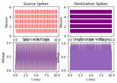
Results from the Second Network

plt.figure()
plt.subplot(2,2,1)
spike_raster_plot(t,data[:][6:6+pop_size],colors=['red'])
plt.ylabel('Neuron')
plt.title('Source Spikes')
plt.subplot(2, 2, 2)
spike_raster_plot(t,data[:][6+2*pop_size:6+3*pop_size],colors=['purple'])
plt.ylabel('Neuron')
plt.title('Destination Spikes')
plt.subplot(2,2,3)
for i in range(pop_size):
    plt.plot(t,data[:][6+pop_size+i])
plt.xlabel('t (ms)')
plt.ylabel('Voltage')
plt.title('Source Voltage')
plt.subplot(2, 2, 4)
for i in range(pop_size):
    plt.plot(t,data[:][6+3*pop_size+i])
plt.xlabel('t (ms)')
plt.ylabel('Voltage')
plt.title('Destination Voltage')

plt.show()